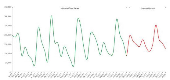
Board provides a Predictive Engine (B.E.A.M.) that will help users in their forecast.
This tool will calculate an automatic forecast based on historical data, through the application of mathematical models that will be automatically adjusted depending on the historical data.

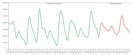
In the picture above you can see an example of historical data (in green) forecasted to the future through the Predictive Analytics functionality (in red).
Though the automatic nature of Predictive Analytics tool, it remains very flexible allowing the user to refine its forecast, adding information to the forecast scenario. In fact, other than the historical time series, the user can feed the B.E.A.M. with other measures and parameters affecting the prediction. The system first understand, which is the best model to be applied to historical data (learning phase), and later applies the model to the coming time periods (forecast phase).
1.1 Basic Concepts
In this section we discuss a series of concepts to better understand the Analytics Interface and use it properly.
1.1.1 The Flow
When you run a Predictive Analytics scenario, on some source cube, the engine will
Detect the time series;
Label each time series as Discontinued, Intermittent or Smooth;
Trim the time series removing the zeroes at the beginning of each series;
Identify the best model for each series via competition;
Identify the outliers;
Detect useful covariate, apply exogenous covariates and discards covariates that do not improve the model.
Serialize the model for future reuse
This part is the learning part, once completed the system applies the model to the future values (forecast horizon) and output various indicators: this part is the forecasting part.
We now explain all the concepts listed above (time series, outliers, covariates…) one by one, please note that this whole process is automatic and the user has no perception of what is happening : he will be notified when the outputs of the process are ready (see below).
1.1.2 Time series
In general a time series is a list of values along a time entity (day, week, month).
Let’s pretend you want to forecast data in a cube (the observed cube) structured by City, Product and Month, but you want to perform the forecast at Region, Product Group and Month level (structure of the target cube). The time series are all the non zero combination of Region and Product Group in the source cube. In other words if in a layout we put Product group and city by row, and month by column, each row will represent a time series.
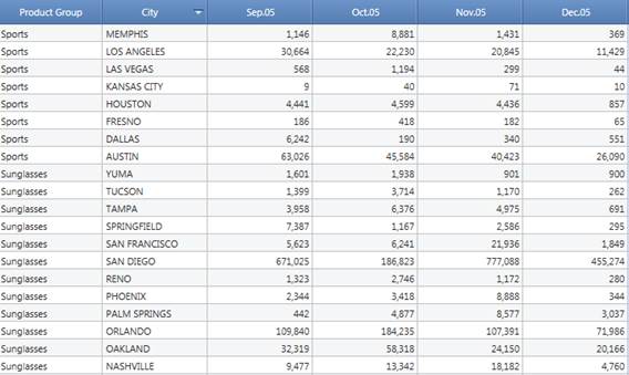
The number of time series is named granularity.
1.1.3 Time series labelling
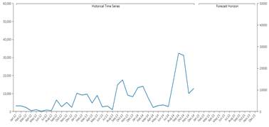
There are three types of time series, discontinued, intermittent and smooth.
Discontinued
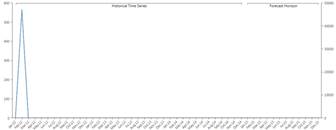
A time series is discontinued if it’s definitively zero (data of the last year is always zero).
Intermittent
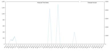
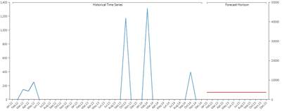
A time series is Intermittent if it’s often zero but has values on some periods. For examples if you are selling big machinery, it’s unlikely that you sell them every month, but most probably twice a year. A series like that is intermittent. Technically we calculate the median time elapsed (in periods) between two non zero values in the series, if this value is greater than 1.3 then the series is intermittent.
Smooth
A series with values on pretty much every period is defined as smooth, basically all the series that are not intermittent or discontinued are smooth (the median time in periods elapsed between two non zero values is less than 1.3).
1.1.4 Models
Discontinued Time series are assumed to be zero also in the future, so the model for this kind of series is just a zero value on every period. Intermittent series will use the Croston-SBA model to be forecasted. Due to the nature of this model the forecast on the future will be a constant on every period.
When it comes to smooth series things are a little bit more complex. The model for time series is named Idsi-ARX. This model is part of the ARIMA family. The arima is fitted to the time series through competition: the series is truncated at 0.75 the length in periods, the first part is used to calculate the ARIMA and the remaining part is used as a benchmark. The model that best fits will be selected. In the competition we will also have the two naïve predictors, the persistent one (constantly the last value of the series) and the seasonal one (basically a previous year). The model that wins the competition is chosen and used to calculate also the future values, using all the data as input. The picture below shows the concept of competition : the green series is predicted with orange and blue series, the blue is closer (in the squared error mean) to the original series, so it’s chosen versus the orange one.

Once the model is chosen the forecast is calculated adopting such model.
1.1.5 Outliers
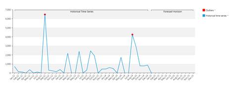
The system also detects anomalous values in the historic data : the so-called "outliers". A time series value is an outlier, if its error against the model is more than 3.5 times the standard deviation.
1.1.6 Covariates
A Covariate is a time series applicable to the entire time horizon (future and past) that is somewhat related to the observed time series. For example, If I’m an Easter-Eggs seller, a series defined as 1 during the easter perido and 0 outside is a covariate. The system evaluates the effect that this covariate had on the series and applies it to the future if and only if the covariate is meaningful : if the inclusion of the covariate's effect in the prediction generates a bigger prediction error the covariate is discarded. A covariate can be a boolean (like the sample's) or another time series (for example the average temperature is a covariate when I am observing the ice creams sales time series). It is not mandatory to set up future values for a covariate: if you know that your store of Easter Eggs was closed during a certain period and this won’t happen in the future you can just tell the system that something happened during that period and it wont happen anymore.
Example 1:
Forecast of Ice creams sales with and without the temperature covariate (forecast period is the 2015).

Example 2:
Promotion Campaigns for ice creams during some particular period (Past and Future Boolean Covariate , forecast period is the 2015)

Example 3:
My ice cream shop closed twice in the past for a whole month, but I don't expect this to happen anymore (Past Boolean Covariate). Green series consider the covariate, blue series don’t.

You can apply as many covariates as you like, there is not a limit.
1.1.7 Prediction intervals
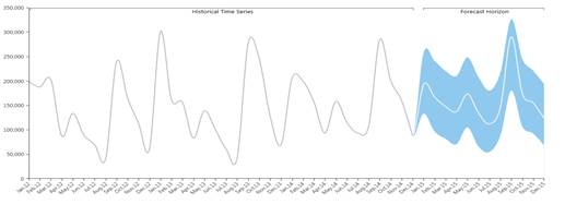
Given a level of confidence X, a prediction interval is a n-time periods of values where predicted values will fall with probability X.
In other words, if we set a level of confidence of 90% the system provides a lower value and an upper value for the forecasted periods. Future observed values will fall between the Low and High values with the 90% of probability .
EXAMPLE:
At the end of 2015 we will observe that 90% of the values have fallen in the blue area of the graph below.
1.1.8 Reconciliation
When you have multi-versions cubes, Predictive Analytics will handle this considering each version a separate scenario.
The sum of the forecasts of the most detailed versions is different from the forecast of the less detailed one, this means that the target cube is not aligned.
You can choose to leave this cube not aligned or to perform reconciliation.
There are two Types of reconciliations: top-down and bottom-up.
Top-Down: it allocates data of the aggregated version to the lowest version (similar to split and splat) proportionally to the lowest version cell values
Bottom-up: it aligns the cube.

1.1.9 Error Statistics
The System computes different types of errors.
MAE (Mean Absolute Error): it is the average of the absolute difference between the observation and their forecast. This measure is scale dependent.
MAPE (Mean Absolute Percentage Error): it is the average absolute percentage size of the error. This measure is scale independent.
MASE (Mean Absolute Scaled Error): It’s the ratio of the MAE and the MAE of the naïve model. It is scale independent and it measures how good the forecast has been compared to the naïve. A MASE grater than 1 indicates that the model selected performed worse than the naïve, if it’s less than 1 the model performed better than the naïve.
Weighted MASE Overall: This measure is the weighted average of all the MASE indicators of the various time series.
For the users with proper license it can be found in the database tab:

The Scenario Configurator opens; check the picture below to understand every section of it:
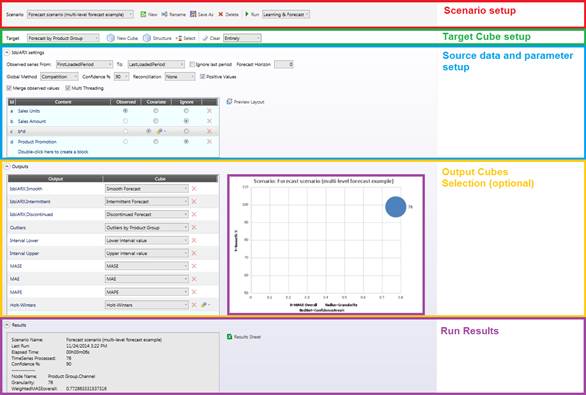
2.1 Scenario Setup
![]()
Select the scenario to edit or run from the drop down list on the left, you can also duplicate a scenario and rename it. The drop down list on the right allows you to decide whether the system should run the learning phase again on every run or only the forecasting phase.
Please note that before the first run it is mandatory to run both learning and forecast, so the drop down list will be grayed out. The only reason to launch a scenario with no learning it’s improving your performance.
2.2 Target cube setting
![]()
Select the cube that gets your forecast data:, the cube must have a dense structure- A new cube can be here created or its structure can be edit. You can have multiple versions.
The Select narrows the series where the prediction calculation runs. Select on Time dimension is not available (please refer to next section).
You can also decide whether to clear the entire cube during the forecast calculation or to clear only the current range .
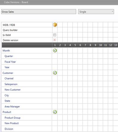
The target cube determines the time dimension and the prediction granularity.
Example:
 a
a
Any populated combination of Customer and Product in the source data will represent a time series, the time series are monthly based.
2.3 Input data and model settings

This section is the most important of the Scenario setup, the accuracy of your forecast mainly depends on the historical data set.
In the two drop down lists you can select which periods will be observed, the default values are
FirstLoadedPeriod: The oldest value in the cube given the selection: please note that this value is unique and it is not evaluated for each time series;
LastLoadedPeriod: The last value in the cube given the selection: please note that this value is unique and it is not evaluated for each time series.
If you think that last period data is not complete you can exclude it flagging the “ignore last period” check-box.
Forecast Horizon: here you can decide the amount of periods you want to forecast, the default 0 value will perform your forecast until the end of the time range.
Global Method: You can decide to get the model via competition or force one of the two Naïve predictors.
Confidence: here you decide the level of confidence to calculate upper and lower interval.
Reconciliation: Select one of the three reconciliation types; this is only needed with multi versions target cubes.
Positive values: Flag this if you want to automatically discard all the models that give some negative result in some period.
Merge observed values: When this setting is on, the historical data will be copied to the target cube along with the forecast.
Multi Threading: This flag won’t affect calculation results, it improves calculation performances on machines supporting multi-threads.
Let’s move to the source layout.
Here you can decide the cubes and algorithms to use as source data.
Cubes and algorithms can be set up as:
Observed: there can be only one observed cube/algorithm this will be the quantity you are going to forecast
Covariate: there can be as many covariate as you like. Covariates are cubes containing time series with values on the entire time horizon that have some sort of impact on the observed series (for example you can use the average temperature by month if you are observing Ice cream sales). You can decide also the maximum lag of the covariate, that’s the maximum number of periods back and forth that will be influenced by a covariate value on a given period. System will discard covariates that do not give any benefit to the forecast; clicking on the gear icon you can force the adoption of the covariate
Ignore,it discards the block.
You can preview this layout clicking the button on the top right corner. It prompts the layout with time period by row.
2.4 Outputs
Other than the forecast in the target cube, Predictive Analytics outputs a lot of data. You can decide to put this data into a series of cube if you need it.
The output cubes are not mandatory like the target cube, their structure will be the same as the target cube (if they have different structures they will be automatically converted).
IdsiARX.Smooth: This cube will be a slice of the target cube that will contain only the smooth time series.
IdsiARX.Intermittent: This cube will be a slice of the target cube that will contain only the intermittent time series.
IdsiARX.Discontinued: This cube will be a slice of the target cube that will contain only the discontinued time series.
Outliers: this cube will only be populated on the past with the anomalous values of the various time series.
Interval lower: this cube will contain the lower limit of the forecast, actual values will be greater than the interval lower and less than the interval upper with a probability equal to the confidence level.
Interval upper: this cube will contain the upper limit of the forecast, actual values will be greater than the interval lower and less than the interval upper with a probability equal to the confidence level.
MASE: Cube containing the MASE of each time series, the MASE of a period is the MASE of the model against the time series until that period.
MAE: Cube containing the MAE of each time series, the MAE of a period is the MAE of the model against the time series until that period.
MAPE: Cube containing the MAPE of each time series, the MAPE of a period is the MAPE of the model against the time series until that period.
Holt-Winters: Also known as triple exponential smoothing, it will output the triple exponential smoothing of the series. The alpha, beta and gamma parameters can be set up directly from the interface. Please note that Holt-Winters is the algorithm beneath the forecast time function in the block editor.
2.5 Run Results
After every run you will get some statistics about the execution time, the number of time series, and the Weighted MASE overall, you’ll also have a graph that will plot the MASE against the number of smooth series.
2.6 Run a scenario via procedure
You can also run a Predictive Analytics scenario from procedure:

The user is allowed to decide whether running the scenario with the procedure selection or the scenario selection and with the learning calculation Y/N.